Linear Regression from Scratch: The Foundation of Machine Learning

Why Linear Regression?

Imagine you’re a real estate analyst trying to predict house prices. You notice a pattern: larger houses tend to cost more. But how do you turn this observation into a precise, mathematical prediction? How do you quantify this relationship?

This is where Linear Regression comes in. It’s not just a statistical method, it’s the gateway to understanding how machines learn patterns from data. Linear Regression forms the foundation that many complex AI systems build upon.

The Core Idea: Finding the Best-Fit Line

At its heart, Linear Regression seeks to find the straight line that best describes the relationship between variables. Think back to high school math: \(y = mx + b\) . In machine learning terms, this becomes:

Where:

• \(y\) is the value we want to predict (the dependent variable)
• \(X\) is the input feature (the independent variable)
• \(W\) is the weight (how much \(X\) influences \(y\))
• \(b\) is the bias (the base value when \(X\) is zero)

The magic lies in finding the perfect \(W\) and \(b\) that make the line fit the data as closely as possible.

The Learning Process: Gradient Descent

But how do we actually find these magical numbers \(W\) and \(b\)? We use an optimization algorithm called Gradient Descent, the workhorse behind many machine learning algorithms.

Here’s the intuition: imagine you’re standing on a mountain and want to find the lowest valley. You look around, feel the slope beneath your feet, and take a step downhill. Repeat this process enough times, and you’ll eventually reach the bottom.

In mathematical terms, the “mountain” is the cost function, a measure of how wrong the predictions are. The slope is the gradient, which points in the direction of steepest ascent. We want to go downhill, so we move in the opposite direction.

The Secret Sauce: Feature Normalization

Before we dive into the code, there’s one crucial concept that makes the algorithm work reliably: feature normalization.

Why do we need it? Imagine the house size data ranges from 650 to 1500 square feet, while prices range from 200,000 to 450,000. These different scales can make gradient descent slow and unstable.

Normalization rescales the features to have a mean of 0 and standard deviation of 1:

X_normalized = (X - self.X_mean) / self.X_std

This ensures all features contribute equally to the learning process and helps gradient descent converge faster.

Code Walkthrough: Building Robust Linear Regression

Let’s examine the actual implementation. This improved version includes feature normalization for better performance:

import numpy as np

class LinearRegression:
    
    def __init__(self, n_iterations=1000, learning_rate=0.001):
        self.n_iterations = n_iterations
        self.learning_rate = learning_rate
        self.W = None
        self.bias = 0
        self.X_mean = None
        self.X_std = None

    def fit(self, X, y):
        n_samples, n_features = X.shape
        
        self.X_mean = np.mean(X, axis=0)
        self.X_std = np.std(X, axis=0)
        X_normalized = (X - self.X_mean) / self.X_std
        
        self.W = np.zeros(n_features)

        for _ in range(self.n_iterations):
            y_pred = np.dot(X_normalized, self.W) + self.bias

            dw = (1 / n_samples) * np.dot(X_normalized.T, (y_pred - y))
            db = (1 / n_samples) * np.sum(y_pred - y)

            self.W -= self.learning_rate * dw
            self.bias -= self.learning_rate * db

    def predict(self, X):
        X_normalized = (X - self.X_mean) / self.X_std
        return np.dot(X_normalized, self.W) + self.bias

Breaking Down the Learning Loop

1. Normalization: We calculate and store the mean and standard deviation of the training data, then transform features to a consistent scale.
2. Initialization: We start with W and b set to zero, a blank slate waiting to learn.
3. Prediction: Using the current W and b, we predict house prices. With normalized features, the initial guesses are more reasonable.
4. Gradient Calculation: (y_pred - y) calculates how far off we were. The gradients dw and db tell us which direction to adjust W and b to reduce error.
5. Parameter Update: We adjust W and b by taking a small step (learning_rate) in the direction that reduces error.

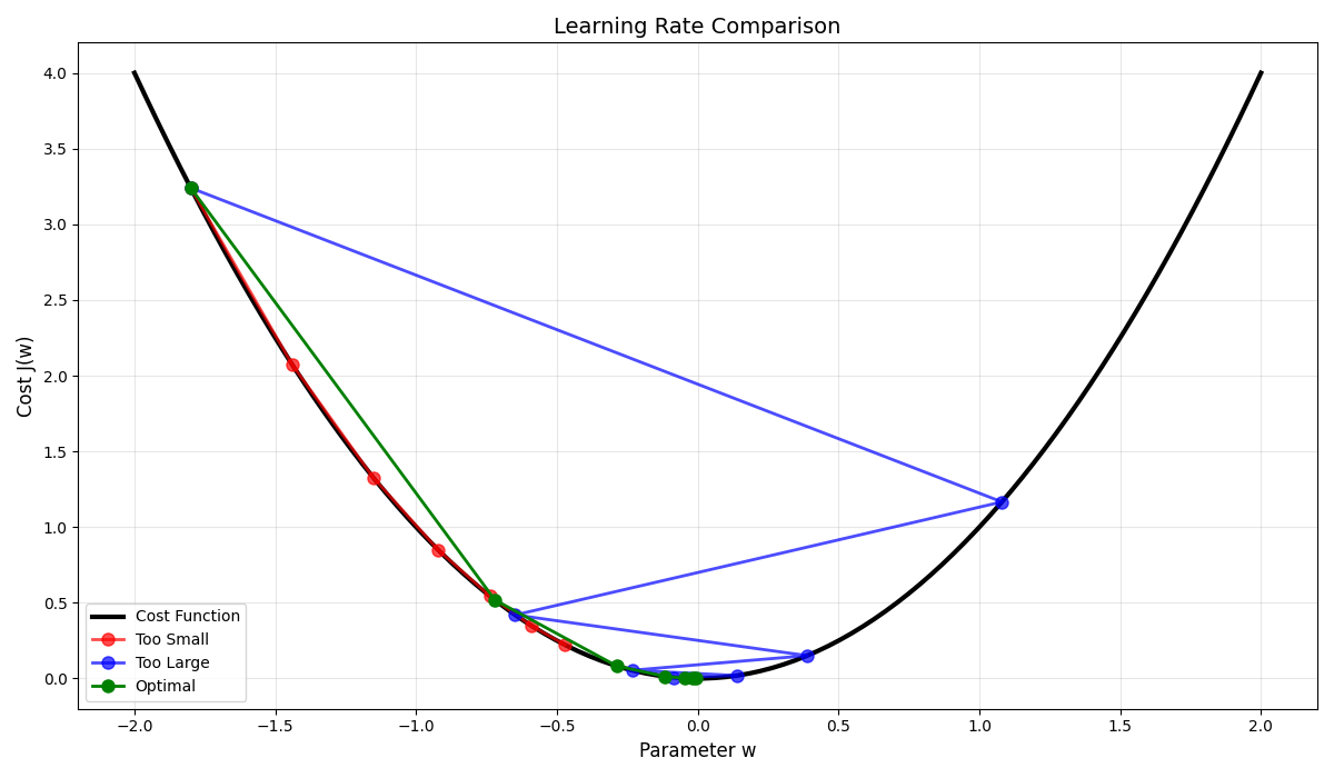
The Importance of the Learning Rate

The learning_rate is a crucial hyperparameter. Too large, and we might overshoot the minimum. Too small, and learning becomes painfully slow. It’s like choosing between taking giant leaps (risking overshooting the valley) or tiny shuffles (taking forever to get there).

Seeing It in Action

Here’s how you’d use the improved Linear Regression class:

if __name__ == "__main__":
    X = np.array([[650], [785], [1200], [1500]])
    y = np.array([200000, 250000, 350000, 450000])

    model = LinearRegression(n_iterations=1000, learning_rate=0.0001)
    model.fit(X, y)

    new_house = np.array([[1000]])
    predicted_price = model.predict(new_house)
    print(f"Predicted price for a 1000 sq ft house: ${predicted_price[0]:.2f}")

The normalization ensures the algorithm works reliably even when features have different scales, a common scenario in real-world data.

Beyond Simple Lines: Multiple Features

While I used one feature (size), real-world problems often involve multiple factors. What about number of bedrooms, location, or age of the house? This implementation naturally handles this:

Each feature gets its own weight, and normalization becomes even more critical when features have different units and scales.

Why These Improvements Matter

The addition of feature normalization transforms the implementation from a theoretical exercise to a practical tool. It addresses key challenges in real machine learning:

• Stable Convergence: Gradient descent works reliably across different datasets

• Faster Training: Normalized features help the algorithm find optimal parameters quicker

• Better Generalization: Consistent feature scaling improves performance on new data

From Theory to Practice

In the implementation, I’ve created more than just a predictor, I’ve built a robust learning system that handles real-world data challenges. The principles I’ve implemented (gradient descent, normalization, iterative learning) form the foundation of much more sophisticated AI systems.

Linear Regression with proper preprocessing demonstrates that successful machine learning isn’t just about complex algorithms, it’s about understanding your data and preparing it properly.

Wrapping Up

Linear Regression is much more than fitting a line through points, it’s your first introduction to how machines learn. By implementing it from scratch, you’ve uncovered the fundamental mechanics that power much of modern AI:

• The iterative nature of parameter optimization
• The crucial role of gradient descent
• The importance of data preprocessing
• How models generalize from training data to make predictions

These concepts scale far beyond linear models. The same principles of gradient-based optimization form the backbone of deep learning networks that power everything from image recognition to natural language processing.

If you want to see the complete implementation and experiment with different datasets:

View the Full Code on GitHub

Try modifying the learning rate, adding polynomial features, or testing with real-world datasets. There’s no better way to understand machine learning than by building it yourself.