Modeling Tennis Matches with Markov Chains

Tennis is deceptively simple on the surface: hit a ball over a net. But beneath that simplicity lies one of the most mathematically rich scoring systems in sports. A single point can feel random, a lucky net cord, a gust of wind, but string together thousands of points, and suddenly the better player almost always wins. How does this deterministic outcome emerge from seemingly random events?

The answer lies in the nested structure of tennis scoring and the powerful mathematical framework of Markov chains. In this post, we’ll journey from a single point to an entire match, building a probabilistic model that explains why small advantages compound dramatically over time.

The Tennis Paradox: Random Points, Deterministic Matches

Consider this: if you flip a fair coin 100 times, you expect roughly 50 heads and 50 tails. But in a best-of-five tennis match, even a player who wins just 52% of points will win the match more than 70% of the time. This “amplification effect” is what makes tennis fascinating from a probability perspective.

The key is hierarchical structure:

Each level builds on the previous one, and at each stage, small advantages get magnified. Let’s see how.

Why Markov Chains Are Perfect for Tennis

A Markov chain is a mathematical system that moves between different “states” with certain probabilities, where the next state depends only on the current one, not on how you got there. This is exactly how tennis works:

• States: The current score (0-0, 15-30, deuce, etc.)
• Transitions: Win or lose the next point with probability \(p\) or \(q = 1-p\)
• Memoryless property: The probability of winning the next point doesn’t depend on the previous rally

For instance, whether you’re at 30-15 because you won three straight points or lost two and won three doesn’t matter, the probability of winning the next point is still \(p\).

This memoryless property is crucial and makes tennis an ideal candidate for Markov chain analysis. In contrast, sports like basketball (where momentum plays a role) or soccer (where tactical adjustments matter) are harder to model this way.

Level 1: From Point to Game

Let’s start with the fundamental unit: a game. To win a game in tennis:

• You must win at least four points
• You must win by at least two points

The scores (0, 15, 30, 40) correspond to (0, 1, 2, 3) points won. We can visualize this as a grid of states:

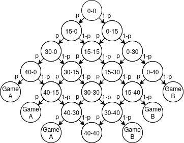
Think of each cell as a possible game state. From (30-15), you can move to (40-15) if you win the point, or (30-30) if you lose it. The question is: starting from (0-0), what’s the probability of reaching “Win” before reaching “Lose”?

The Mathematics of Winning a Game

Let \(P(a, b)\) be the probability that Player A wins the game when the score is \(a\) points for A and \(b\) points for B. We can write a recursive relationship:

where \(p\) is the probability of winning the next point and \(q = 1 - p\).

This says: “The probability of winning from \((a, b)\) is the probability of winning the next point times the probability of winning from the next state if we win, plus the probability of losing the next point times the probability of winning from the next state if we lose.”

The boundary conditions are:

• If \(a \geq 4\) and \(a - b \geq 2\), then \(P(a, b) = 1\) (we’ve won)
• If \(b \geq 4\) and \(b - a \geq 2\), then \(P(a, b) = 0\) (we’ve lost)

The Deuce Problem: An Infinite Loop

But there’s a catch. When both players reach 40-40 (deuce), the game doesn’t end until someone wins by two. This creates a potential infinite loop:

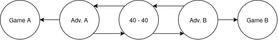
From deuce, you can:

• Win two straight points \(\rightarrow\) Game won (probability \(p^2\))
• Lose two straight points \(\rightarrow\) Game lost (probability \(q^2\))
• Split the next two points \(\rightarrow\) Back to deuce (probability \(2pq\))

This loop can theoretically continue forever! To find the probability of eventually winning from deuce, \(P_D\), we use a clever trick. Let’s write an equation:

This says: “The probability of winning from deuce equals the probability of winning two straight points, plus the probability of returning to deuce times the probability of winning from deuce.”

Solving for \(P_D\):

Notice something beautiful: if \(p = 0.5\) (perfectly even players), then \(P_D = 0.5\). But even a tiny advantage (say \(p = 0.52\)) gives \(P_D \approx 0.519\), a noticeable edge in a potentially long deuce battle.

Putting It All Together

The complete formula for winning a game combines:

1. Direct wins (winning 4-0, 4-1, 4-2)
2. Deuce scenarios (reaching 3-3 and then resolving via \(P_D\))

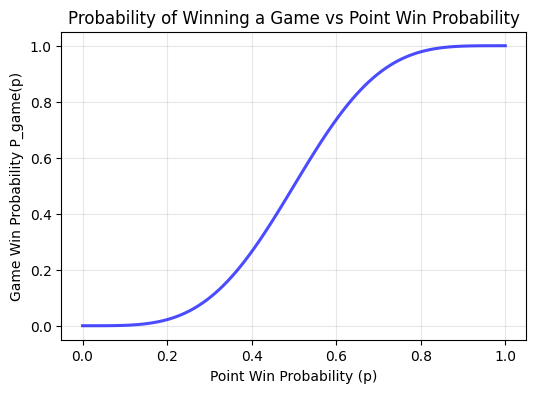
Look at this curve! Even at \(p = 0.6\) (winning 60% of points), you win the game about 80% of the time. This is the first level of probability amplification.

Level 2: From Game to Set

Now we climb one level higher. A set is typically won by:

• The first player to win six games
• With a lead of at least two games
• If it’s 6-6, there’s usually a tiebreak (which we’ll simplify for now)

The logic is identical to the game level, but now our “point” is a game, and our probability is \(P_{\text{game}}(p)\). Let’s call this \(g\) for short.

The Set-Level Markov Chain

We can write a similar recursive formula:

where \(a\) and \(b\) are the number of games won by each player.

Again, we have:

• Boundary conditions for winning/losing
• A “set deuce” scenario at 5-5

The formula becomes:

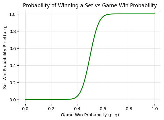
Notice the curve is even steeper than the game curve. If you win 60% of games, you win about 90% of sets. The advantage is compounding!

Level 3: From Set to Match

Finally, the match level. In professional tennis, men play best-of-five sets (in Grand Slams) or best-of-three (most other tournaments). Women typically play best-of-three.

This is the simplest level mathematically because there’s no “deuce”, you either win 2 out of 3 sets (or 3 out of 5).

Best of 3

where \(s = P_{\text{set}}(g)\).

This formula accounts for:

• Winning 2-0 (probability \(s^2\))
• Winning 2-1 (probability \(2s^2(1-s)\))

Best of 5

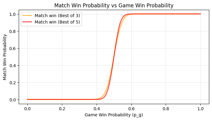
The amplification effect is now extreme. If you win 55% of points (barely better than a coin flip), you win:

• ~75% of games
• ~88% of sets
• ~93% of best-of-three matches
• ~96% of best-of-five matches

The Full Picture: From 55% to 96%

Let’s put everything together and see the complete amplification chain:

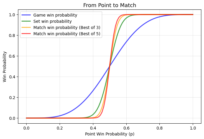
This graph reveals why tennis feels so “fair”, the better player almost always wins, even if their advantage per point is tiny. It also explains why:

• Grand Slam champions (BO5 format) tend to be the truly elite players
• Early-round upsets are rarer in tennis than in single-elimination sports like the NCAA tournament
• Serve dominance matters so much (we’ll explore this in a future post)

Real-World Implications

This model has practical applications:

• Betting markets: Understanding how point-level statistics translate to match outcomes
• Player analysis: Quantifying how much a serve improvement would increase match win rate
• Tournament seeding: Why protecting top seeds makes mathematical sense
• Training focus: Small improvements in consistency (increasing \(p\) from 0.51 to 0.53) have outsized effects

What We Haven’t Covered (Yet)

This model assumes all points are equally likely to be won. But tennis is more subtle:

• Serving gives a massive advantage (pros win ~65% of service points vs ~35% of return points)
• Momentum might exist (though statisticians debate this)
• Psychological factors like pressure on break points
• Tiebreaks have different dynamics

In the next post, we’ll extend this model to account for serve/return asymmetry, which adds another layer of realism and reveals why “holding serve” is so critical.

Conclusion

Tennis scoring is a masterclass in probability amplification. The nested structure (points \(\rightarrow\) games \(\rightarrow\) sets \(\rightarrow\) matches) transforms small advantages into near-certainties. Markov chains provide the perfect mathematical framework for understanding this amplification, revealing the elegant determinism hidden beneath the apparent randomness of individual points.

The beauty of this model lies in its simplicity: with just one parameter (the probability of winning a point), we can predict match outcomes with surprising accuracy. Yet it also points to deeper complexity: the model suggests that tennis is purely “memoryless,” but any tennis fan knows that momentum, pressure, and psychology play roles too. Those factors are harder to quantify, but they make the sport all the more fascinating.

Repository and Code

All formulas, derivations, and visualizations from this post come from the Tennis Markov notebook. You can explore the complete implementation here:

GitHub Repository: tennis-markov

The notebook includes:

• Complete derivations of all formulas
• Interactive visualizations
• Monte Carlo simulations to verify the math (Coming soon)
• Extensions for tiebreaks and other scenarios (Coming soon)

Next post preview:
In the next entry, we’ll break the symmetry assumption and model serving vs. returning, exploring how the server’s advantage changes the entire probability landscape. We’ll also look at how the “break point” becomes one of the most critical moments in a match from a mathematical perspective.