K-Means Clustering from Scratch: Grouping Data with Python

The Art of Finding Order in Unlabeled Data

Most machine learning tutorials start with supervised learning, predicting prices, classifying images, or recognizing spam. But what about the vast majority of data that comes without labels? What if you have customer information but no predefined segments, or documents but no categories?

This is where unsupervised learning shines, and K-Means clustering stands as its most intuitive and widely-used algorithm. It’s the tool that helps machines discover the natural groupings that exist in your data, much like how humans naturally categorize things without being explicitly taught.

The Beautiful Simplicity of K-Means

At its core, K-Means solves a problem that seems almost philosophical: how do you find structure where none is apparent? The answer lies in a beautifully simple iterative process that even humans use intuitively.

Imagine you’re an archaeologist who just discovered 100 ancient coins. You suspect they come from different historical periods, but you have no documentation. How would you group them?

1. You’d first pick K coins that seem representative of different eras
2. You’d compare each remaining coin to these representatives and group them with the most similar one
3. For each group, you’d calculate a new “average” representative coin
4. You’d repeat this process until the groups stop changing

This is exactly what K-Means does, but with mathematical precision.

The Mathematical Intuition: Alternating Optimization

K-Means works by solving what’s known as an alternating optimization problem. It breaks down a complex challenge into two simpler sub-problems that it solves repeatedly:

1. Cluster Assignment: Given fixed centroids, assign each point to the closest center
2. Centroid Update: Given fixed cluster assignments, compute the optimal centers

This approach is powerful because each step is easy to solve, and repeating them leads to a good overall solution. It’s like having two experts who take turns improving the result, one focusing on group membership, the other on group representation.

Code Deep Dive: Building the K-Means Engine

Let’s examine the key components that make the implementation work. The heart of the algorithm lives in the predict method:

def predict(self, X):
    centroids = self._initialize_centroids(X)
    
    for _ in range(self.max_iter):
        clusters = self._assign_clusters(X, centroids)
        
        previous_centroids = centroids
        
        centroids = self._update_centroids(X, clusters)

        diff = np.linalg.norm(centroids - previous_centroids)
        if diff < EPSILON:
            break

    return self._get_labels(X, clusters)

The Distance Measure: Defining “Closeness”

The concept of “closest” is fundamental to K-Means. I use Euclidean distance, which gives us the straight-line distance between points:

def _euclidian_distance(self, X_1, X_2):
    return np.sqrt(np.sum((X_1 - X_2) ** 2))

This simple formula is what allows the algorithm to form spherical clusters. In high-dimensional spaces, this becomes the foundation for understanding similarity.

The Assignment Step: Finding Where Each Point Belongs

This is where each data point “votes with its feet” and joins the cluster whose center is most similar:

def _assign_clusters(self, X, centroids):
    clusters = [[] for _ in range(self.k)]
    
    for sample_index, sample in enumerate(X):
        centroid_index = self._get_closest_centroid(sample, centroids)
        clusters[centroid_index].append(sample_index)

    return clusters

Notice how I store indices rather than the actual data points, this is both memory-efficient and makes the update step straightforward.

The Update Step: Letting the Centers Adapt

After all points have chosen their groups, the cluster centers recalibrate to become the true center of their members:

def _update_centroids(self, X, clusters):
    n_features = np.shape(X)[1]
    centroids = np.zeros((self.k, n_features))
    
    for i, cluster in enumerate(clusters):
        centroid = np.mean(X[cluster], axis=0)
        centroids[i] = centroid
    
    return centroids

This step is crucial, it’s where the algorithm “learns” what each cluster really represents by listening to its members.

The K-Selection Problem: How Many Groups Are There?

The biggest challenge with K-Means isn’t the algorithm itself, it’s choosing the right value for K. How do you know how many natural clusters exist in your data?

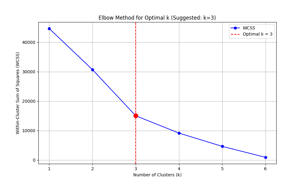
The Elbow Method: Finding the Sweet Spot

I solve this using the Elbow Method, which balances cluster cohesion against model complexity:

@staticmethod
def calculate_wcss(X, max_k=10):
    wcss_values = []
    
    for k in range(1, max_k + 1):
        kmeans = KMeans(k=k, max_iter=100)
        labels = kmeans.predict(X)
        wcss = 0
        
        for cluster_label in range(k):
            cluster_points = X[labels == cluster_label]
            if len(cluster_points) > 0:
                cluster_centroid = np.mean(cluster_points, axis=0)
                distances = np.sum((cluster_points - cluster_centroid) ** 2, axis=1)
                wcss += np.sum(distances)
        
        wcss_values.append(wcss)
    
    return wcss_values

The WCSS (Within-Cluster Sum of Squares) measures how tight the clusters are. As K increases, WCSS naturally decreases, but we look for the point where adding more clusters doesn’t give us much improvement, the “elbow.”

Automating the Elbow Detection

Finding the elbow visually can be subjective, so I automate it by looking for the point of maximum curvature:

@staticmethod
def find_optimal_k_elbow(wcss_values):
    first_derivatives = []
    for i in range(1, len(wcss_values)):
        derivative = wcss_values[i-1] - wcss_values[i]
        first_derivatives.append(derivative)
    
    second_derivatives = []
    for i in range(1, len(first_derivatives)):
        second_derivative = first_derivatives[i-1] - first_derivatives[i]
        second_derivatives.append(second_derivative)
    
    optimal_k = np.argmax(second_derivatives) + 2
    return optimal_k

Seeing the Algorithm in Action: Customer Segmentation

Let’s walk through a complete example using synthetic customer data:

if __name__ == "__main__":
    customer_data = np.array([
        [15, 39], [15, 81], [16, 6], [16, 77], [17, 40], 
        [65, 25], [65, 80], [66, 27], [67, 85], [70, 90],
        [120, 5], [120, 80], [122, 10], [125, 75], [130, 8]
    ])

    print("Step 1: Finding the optimal number of clusters...")
    wcss_values, optimal_k = KMeans.plot_elbow_method(X=customer_data, max_k=6)
    
    print("\nWCSS values for different k:")
    for k, wcss in enumerate(wcss_values, 1):
        print(f"k={k}: WCSS = {wcss:.2f}")

    print(f"\nStep 2: Running K-Means with k={optimal_k}...")
    kmeans = KMeans(k=optimal_k, max_iter=100)
    labels = kmeans.predict(customer_data)

    print("Step 3: Visualizing the results...")
    colors = ['red', 'blue', 'green', 'orange', 'purple', 'brown']
    for i in range(len(customer_data)):
        plt.scatter(customer_data[i, 0], customer_data[i, 1], 
                    color=colors[int(labels[i])], s=100, alpha=0.7)

    plt.xlabel('Annual Income ($ thousands)')
    plt.ylabel('Spending Score')
    plt.title(f'Customer Segments Discovered by K-Means (k={optimal_k})')
    plt.grid(True, alpha=0.3)
    plt.show()

When you run this, you’ll likely see the algorithm suggest K=3, revealing clear customer segments:

• Cluster 1 (Red): Low income, mixed spending
• Cluster 2 (Blue): Medium income, high spending
• Cluster 3 (Green): High income, low spending

The Limitations and Strengths

Like any algorithm, K-Means has its trade-offs:

Strengths:

• Simple to understand and implement
• Efficient on large datasets
• Guaranteed to converge
• Easily adaptable to new data

Limitations:

• Requires specifying K in advance
• Sensitive to initial centroid placement
• Assumes spherical clusters of similar size . Can converge to local optima

In practice, we often run K-Means multiple times with different random initializations to mitigate the local optima problem.

Beyond the Basics: Where K-Means Powers Modern AI

While K-Means seems simple, it forms the foundation for more advanced techniques and appears in surprising places:

• Image Compression: By treating pixels as points in RGB space, K-Means can reduce color palettes
• Document Clustering: Grouping similar articles or research papers
• Anomaly Detection: Points far from any centroid might be outliers
• Feature Engineering: Cluster labels can become features for supervised models
• Market Segmentation: Exactly like the customer example, but with real business data

Wrapping Up: The Beauty of Simple Algorithms

K-Means demonstrates a profound truth in machine learning: sometimes the most powerful insights come from simple, well-executed ideas. By implementing it from scratch, you’ve not just learned an algorithm, you’ve internalized the concept of iterative optimization, the importance of distance metrics, and the art of model selection.

The principles you’ve seen here, alternating optimization, convergence criteria, the bias-variance tradeoff in choosing K, extend far beyond clustering. They’re fundamental concepts that will serve you well as you explore more complex algorithms.

Ready to experiment with your own data?

View the Full Code on GitHub

Try running it on the classic Iris dataset, or better yet, on some unlabeled data from your own projects. There’s nothing quite like seeing an algorithm you built yourself discover patterns that were hidden in plain sight.